Plots the main condvis display

The section plot relates a fit or fits to one or two predictors (sectionvar), for fixed values of other predictors in conditionvals.

sectionPlot(
  CVdata,
  CVfit = NULL,
  response = NULL,
  preds,
  sectionvar,
  conditionvals,
  pointColor = "steelblue",
  sim = NULL,
  threshold = 1,
  linecols = NULL,
  dataplot = "pcp",
  gridsize = 50,
  probs = FALSE,
  view3d = FALSE,
  theta3d = 45,
  phi3d = 20,
  xlim = NULL,
  ylim = NULL,
  zlim = NULL,
  pointSize = 1.5,
  predictArgs = NULL,
  resetpar = TRUE,
  density = FALSE,
  showdata = density == FALSE,
  returnInfo = FALSE,
  pointColorFromResponse = FALSE,
  pcolInfo = NULL
)

Arguments

CVdata

the dataset used for the fit

CVfit

a fit or list of fits

response

name of response variable

preds

names of predictors

sectionvar

section variable, or variables.

conditionvals

conditioning values. A vector/list or dataframe with one row

pointColor

a color, vector of colors,or the name of variable to be used for coloring

sim

vector of similarity weights

threshold

used for similarity weights, defaults to 1.

linecols

vector of line colours

dataplot

"pcp" or "pairs". Used when there is no response, or more than two sectionvars.

gridsize

used to construct grid of fitted values.

probs

Logical; if TRUE, shows predicted class probabilities instead of just predicted classes. Only available with two numeric sectionvars and the model's predict method provides this.

view3d

Logical; if TRUE plots a three-dimensional regression surface if possible.

theta3d, phi3d

Angles defining the viewing direction. theta3d gives the azimuthal direction and phi3d the colatitude. Seepersp.

xlim

passed on to plot

ylim

passed on to plot

zlim

passed on to plot

pointSize

used for points

predictArgs

a list with one entry per fit, giving arguments for predict

resetpar

When TRUE (the default) resets pars after drawing.

density

default FALSE. Use TRUE if model is a density function.

showdata

If FALSE, data on section not shown.

returnInfo

If TRUE, returns coordinates for some plots

pointColorFromResponse

ignore--For interactive use only

pcolInfo

ignore--For interactive use only

Value

plotted coordinates, for some plots

Details

The type of plot depends on the fit and the section variables. Observations with non zero values of the similarity weights sim are shown. If no fit is provided, the data are shown as a parallel coordinate plot or pairs plot, depending on dataplot. The fit could also be a density estimate.

Examples

#Fit a model. 
f <- lm(Fertility~ ., data=swiss)
svar <- "Education"
preds <- variable.names(f)[-1]
sectionPlot(swiss,f, "Fertility",preds,svar, swiss[12,])

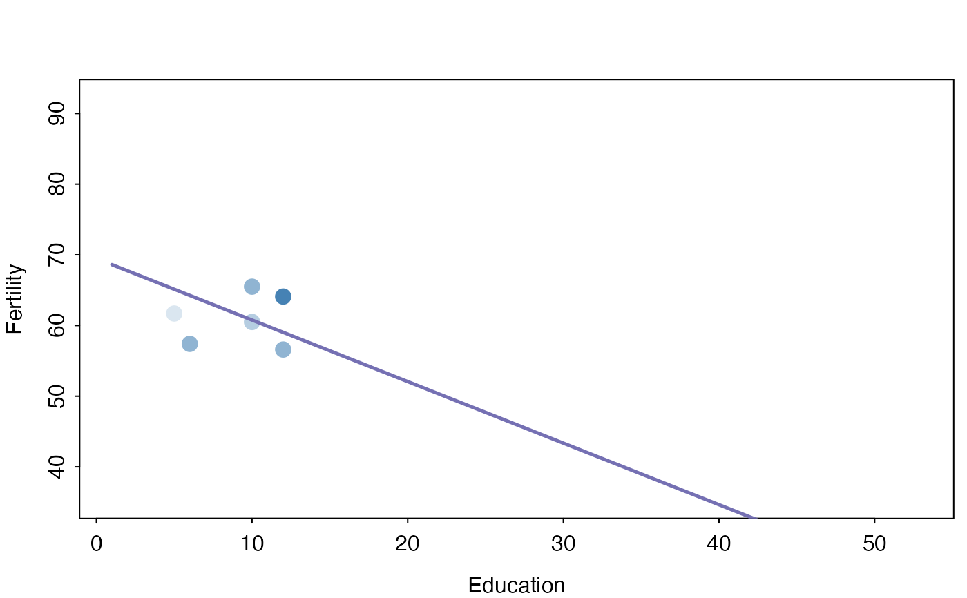sectionPlot(swiss,f, "Fertility",preds,svar, apply(swiss,2,median))

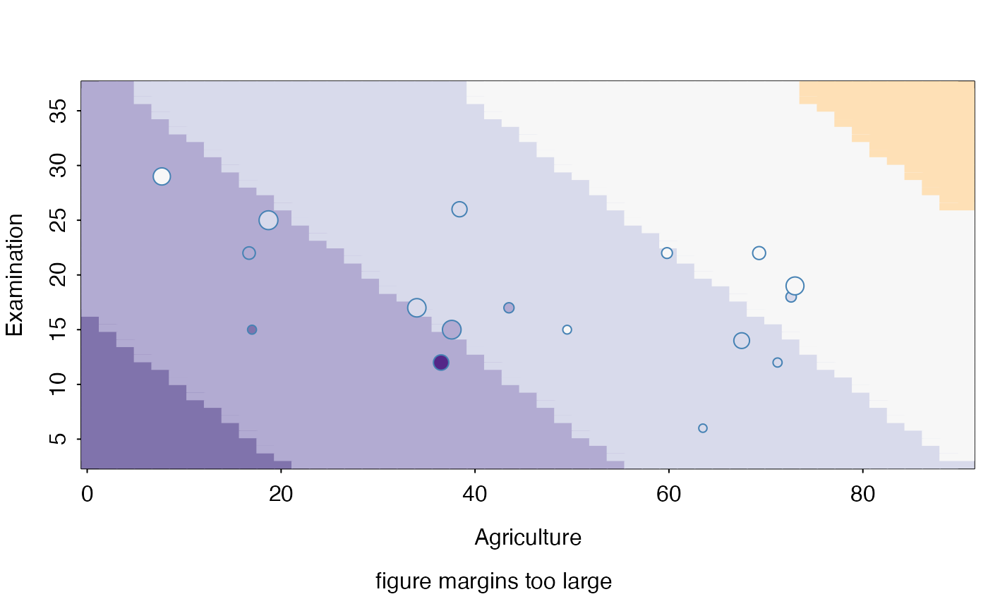
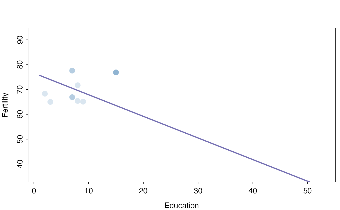sectionPlot(swiss,f, "Fertility",preds,preds[1:2], apply(swiss,2,median))

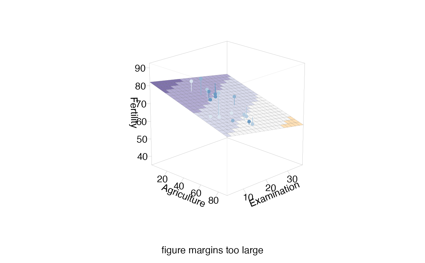
sectionPlot(swiss,f, "Fertility",preds,preds[1:2], apply(swiss,2,median), view3d=TRUE)


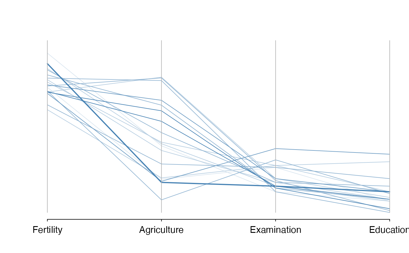
# PCP of swiss data, showing only cases whose percent catholic and infant.mortality are
# similar to those of the first case
sectionPlot(swiss,preds=names(swiss),
           sectionvar= names(swiss)[1:4],conditionvals=swiss[1,] )     

# Use dataplot="pairs" to switch to a pairs plot

# A density estimate example
 if (FALSE) {
 library(ks)
fde <-kde(iris[,1:3])
sectionPlot(iris,list(kde=fde), response=NULL,
           preds=names(iris)[1:3],
           sectionvar=names(iris)[1],
           conditionvals=iris[1,],density=TRUE)
 }